Dodatkowe materiały

• Darmowy kurs MOOC Pogromcy Danych
• Data Wrangling with dplyr and tidyr
• Data frames
• Databases
• Hybrid evaluation
• Introduction to dplyr
• Adding a new SQL backend
• Non-standard evaluation
• Two-table verbs
• Window functions and grouped mutate/filter

RTCGA

source("https://bioconductor.org/biocLite.R") 
biocLite('RTCGA.rnaseq')
biocLite('RTCGA.clinical')
biocLite('RTCGA.mutations')

The Cancer Genome Atlas (TCGA) is a comprehensive and coordinated effort to accelerate our understanding of the molecular basis of cancer through the application of genome analysis technologies, including large-scale genome sequencing.

library(RTCGA.rnaseq); data(BRCA.rnaseq) # information about genes' expressions
library(RTCGA.mutations); data(BRCA.mutations) # information about genes' mutations
library(RTCGA.clinical); data(BRCA.clinical) # patients' clinical data
BRCA.rnaseq %>%
    select(`TP53|7157`, bcr_patient_barcode) %>%
    # bcr_patient_barcode contains a key to merge patients between various datasets
    rename(TP53 = `TP53|7157`) %>%
    filter(substr(bcr_patient_barcode, 14, 15) == "01" ) %>% 
    # 01 at the 14-15th position tells these are cancer sample
    mutate(bcr_patient_barcode = substr(as.character(bcr_patient_barcode),1,12)) -> 
    # in clinical info bcr_patient_barcode is only of length 12
    BRCA.rnaseq.TP53

BRCA.mutations %>%
    select(Hugo_Symbol, bcr_patient_barcode) %>%
    # Hugo_symbol tells to which gene the row corresponds.
    # Ff the rows exist for a gene, this means there was a mutation 
    # for this patient for this gene.
    filter(nchar(bcr_patient_barcode)==15) %>%
    # sometime there are inproper lengths of this code
    filter(substr(bcr_patient_barcode, 14, 15)=="01") %>%   
    # 01 at the 14-15th position tells these are cancer sample
    filter(Hugo_Symbol == 'PIK3CA') %>%
    # we are interested only in the mutations of PIK3CA
    unique() %>% 
    # sometimes there are few mutations in the same gene
    mutate(bcr_patient_barcode = substr(as.character(bcr_patient_barcode),1,12)) -> 
    # in clinical info bcr_patient_barcode is only of length 12
    BRCA.mutations.PIK3CA

BRCA.clinical %>%
    select(patient.bcr_patient_barcode,
           patient.vital_status, # information whether patient is still alive
           patient.days_to_last_followup, # how many days has patient been observed if he is alive
           patient.days_to_death) %>% # how many days has patient been observed if he has passed away
    mutate(bcr_patient_barcode = toupper(as.character(patient.bcr_patient_barcode))) %>%
    # in clinical datasets the key column is in lower case and with different name
    mutate(status = ifelse(as.character(patient.vital_status) == "dead",1,0),
           times = ifelse( 
                        !is.na(patient.days_to_last_followup),
                        as.numeric(as.character(patient.days_to_last_followup)),
                        as.numeric(as.character(patient.days_to_death))
            )) %>%
    # if the patient does not have a days_to_last_followup time this means
    # he has days_to_death time
    mutate(times = as.numeric(times)) %>%
    filter(!is.na(times)) %>% 
    # sometime patient does not have any time
    filter(times > 0) -> BRCA.clinical.survival
    # sometimes by mistkae patients have non-positive times (few cases)

BRCA.rnaseq.TP53 %>%
    left_join(y = BRCA.mutations.PIK3CA,
                        by = "bcr_patient_barcode") %>%
    left_join(y = BRCA.clinical.survival,
                        by = "bcr_patient_barcode") %>%
    mutate(TP53_HighExpr = ifelse(TP53 >= median(TP53), "1", "0")) %>%
    mutate(PIK3CA_Mut = as.integer(!is.na(Hugo_Symbol))) %>%
    select(times, status, TP53_HighExpr, PIK3CA_Mut)  %>%
    filter(!is.na(status)) -> BRCA.2survfit

dim(BRCA.2survfit)

[1] 1040    4

BRCA.2survfit %>%
  group_by(TP53_HighExpr, PIK3CA_Mut, status) %>%
  summarise(counts = n()) %>%
  arrange(desc(counts))

Source: local data frame [8 x 4]
Groups: TP53_HighExpr, PIK3CA_Mut [4]

  TP53_HighExpr PIK3CA_Mut status counts
          (chr)      (int)  (dbl)  (int)
1             0          0      0    359
2             0          0      1     35
3             0          1      0    118
4             0          1      1      9
5             1          0      0    298
6             1          0      1     47
7             1          1      0    161
8             1          1      1     13

BRCA.2survfit %>%
  group_by(TP53_HighExpr, PIK3CA_Mut) %>%
  summarize(min = min(times),
            median = median(times),
            mean = mean(times),
            max = max(times)) -> agr_stats

library(tidyr)
agr_stats %>%
  select(-PIK3CA_Mut) %>%
  top_n(1, max) %>%
  gather(TP53_HighExpr) -> agr_stats_2viz

names(agr_stats_2viz)[2:3] <- c("statistics", "value")
library(ggplot2)
agr_stats_2viz %>%
  ggplot(aes(statistics, value,  group =TP53_HighExpr, col = TP53_HighExpr)) + 
  geom_line() +
  theme_RTCGA()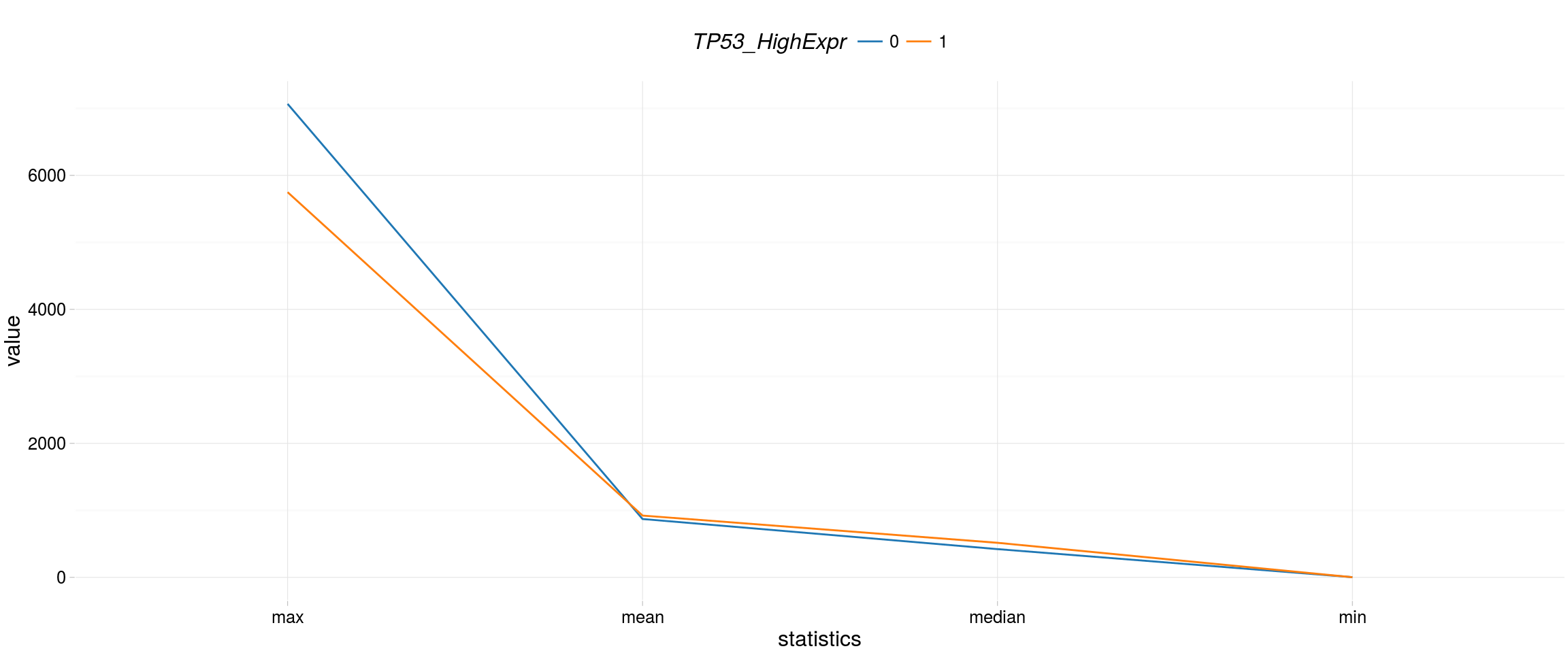

library(survminer)
library(survival)
fit <- survfit(Surv(times, status) ~ TP53_HighExpr + PIK3CA_Mut,
               data = BRCA.2survfit)
ggsurvplot(fit, theme = theme_RTCGA(), p.val = TRUE, risk.table = TRUE,
           risk.table.y.text.col = TRUE, risk.table.y.text = FALSE)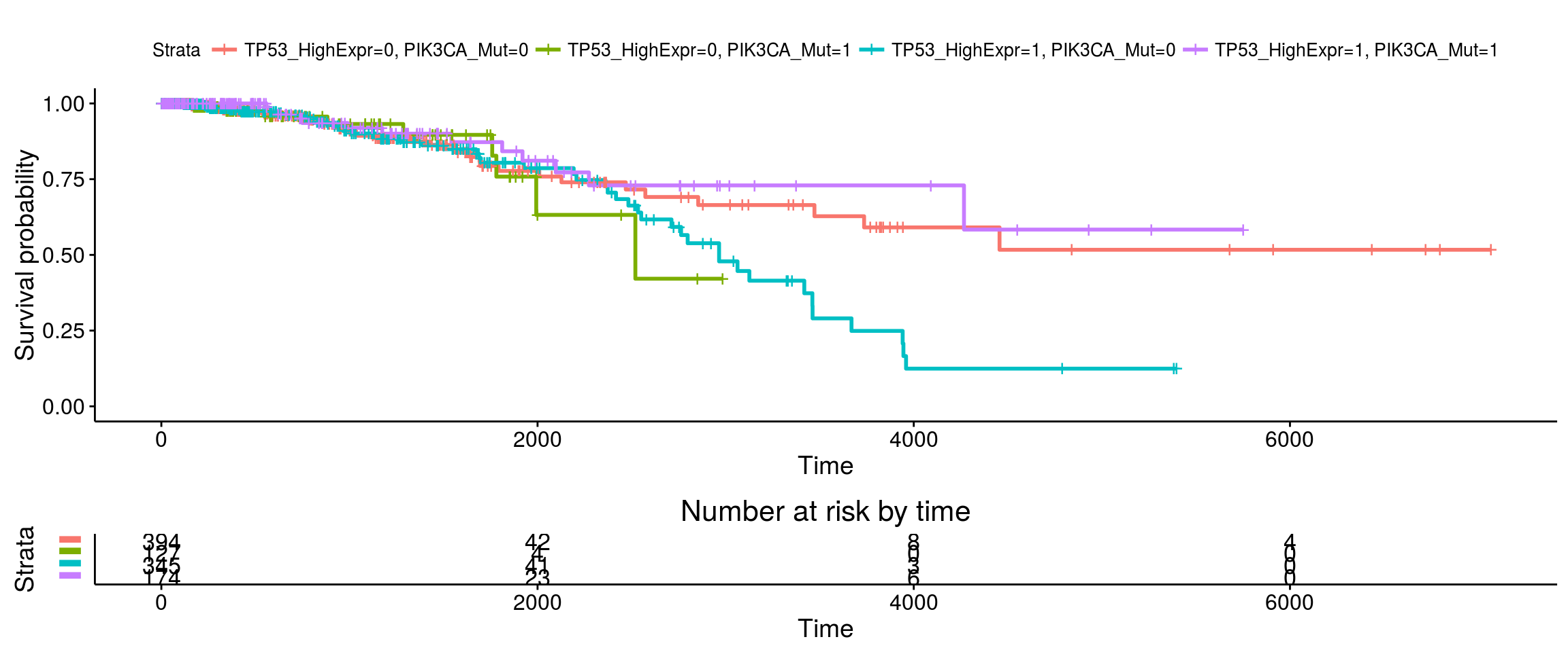

Internet Advertisements Data Set

This dataset represents a set of possible advertisements on Internet pages. The features encode the geometry of the image (if available) as well as phrases occuring in the URL, the image’s URL and alt text, the anchor text, and words occuring near the anchor text. The task is to predict whether an image is an advertisement (“ad”) or not (“nonad”).

Wymiary: 3279 X 1558

ad <- read.csv("~/pg-Rworkshop-2016/dane/ad.data", header=FALSE,stringsAsFactors = FALSE)
ad[ad == "   ?"] <- 0

for(i in 1:ncol(ad)){
  gsub(" ", "", ad[, i]) %>%
    as.character() %>%
    as.numeric() -> ad[, i]
}


ad %>% 
  summarise_each(funs(mean)) %>%
  .[, 1:6]

FSelector - information.gain

library(RTCGA.rnaseq)
library(dplyr)
BRCA.rnaseq %>%
  mutate(bcr_patient_barcode = substr(bcr_patient_barcode, 14, 14)) -> BRCA.rnaseq.tumor
BRCA.rnaseq.tumor.first<-BRCA.rnaseq.tumor[, 1:1000]

(sum(BRCA.rnaseq.tumor.first$bcr_patient_barcode==0))  #1100 guz 

[1] 1100

(sum(BRCA.rnaseq.tumor.first$bcr_patient_barcode==1))  #112 zdrowy

[1] 112

library(FSelector)
information.gain(formula =bcr_patient_barcode~., data = BRCA.rnaseq.tumor.first)->wynik.info

wynik.info %>%
  mutate(nazwy = row.names(wynik.info)) %>%
  arrange(desc(attr_importance)) -> wyniki.po.info

(subset<- cutoff.biggest.diff(wynik.info))

[1] "ADAMTS5|11096"  "ARHGAP20|57569"

(subset)  ##geny o najbardziej wyróżniającym się wskaźniku attr_imprortance

[1] "ADAMTS5|11096"  "ARHGAP20|57569"

(subset11<-cutoff.k(wynik.info,10))

 [1] "ADAMTS5|11096"  "ARHGAP20|57569" "ABCA10|10349"   "ABCA9|10350"    "ALDH1A2|8854"   "ABCA8|10351"    "ADRB2|154"      "ABCA6|23460"   
 [9] "ANKRD29|147463" "AQP7P1|375719" 

Boruta - Boruta

library(Boruta)
invisible(
Boruta_model <- Boruta(as.factor(bcr_patient_barcode)~.,
                       data = BRCA.rnaseq.tumor.first[,1:100], 
                       doTrace =2, ntree = 50)
)
plot(Boruta_model, las=2, xlab="")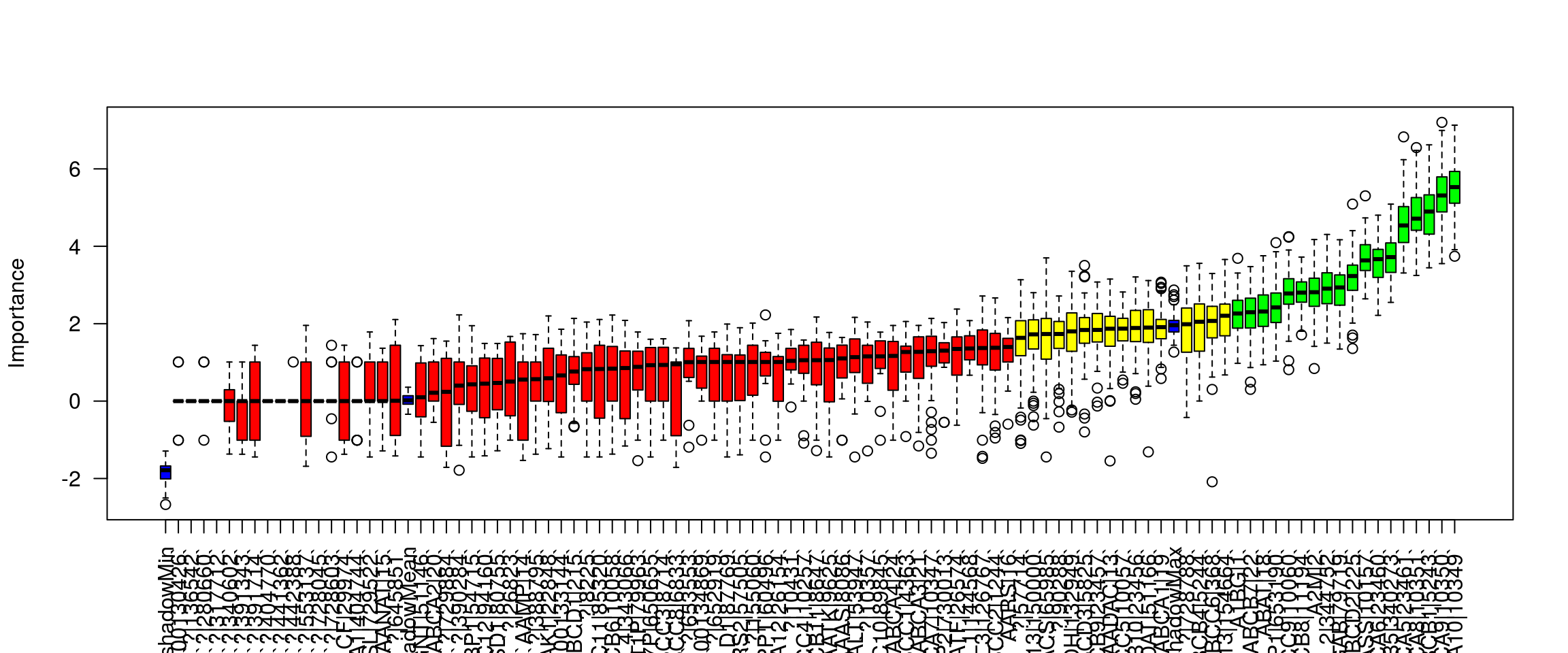

# plotImpHistory(Boruta_model)
# getSelectedAttributes

Regresja logistyczna z regularyzacją

• glmnet poprzez regularyzację sam dobiera odpowiednie parametry

library(glmnet)
model_glmnet <- glmnet(x = as.matrix(BRCA.rnaseq.tumor.first[, -1]),
                       y = as.factor(BRCA.rnaseq.tumor.first[,1]),
                       family="binomial",
                       alpha = 0, lambda.min = 1e-4)
nsteps <- 10
b1 <- coef(model_glmnet)[-1, 1:nsteps]
w <- nonzeroCoef(b1)
b1 <- as.matrix(b1[w, ])
matplot(1:nsteps, t(b1), type = "o", pch = 19,
        col = "blue", xlab = "Step",
        ylab = "Coefficients", lty = 1)
title("Lasso")
abline(h = 0, lty = 2)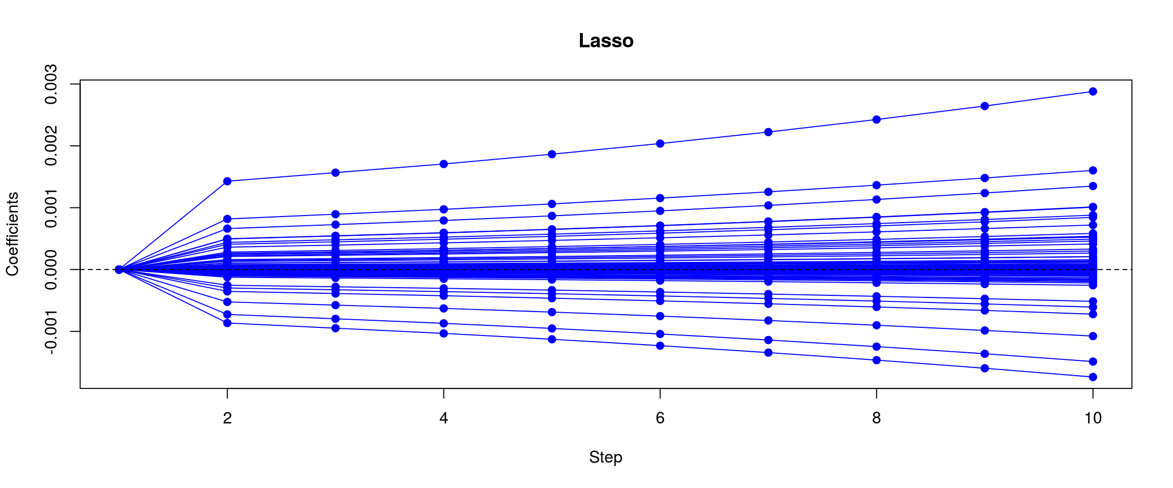

Lasy losowe / drzewa klasyfikacyjne

pakiet caret

• http://topepo.github.io/caret/varimp.html

Funkcje pomocnicze

Do oceny jakości klasyfikatorów przydzadzą się poniższe funkcje

library(ROCR)
tabela <- function(predykcja_klasy, klasy_prawdziwe){
    table(predykcja_klasy, klasy_prawdziwe)
}

procent <- function(t){
    100*sum(diag(t))/sum(t)
}

czulosc <- function(t){
    if(sum(t[2,])==0) return(0) else t[2,2]/(sum(t[2,]))
}

precyzja <- function(t){
    if(sum(t[,2])==0) return(0) else t[2,2]/sum(t[,2])
}

roc <- function(pred_prawdopod, prawdziwe_klasy,...){
    pred <- prediction(pred_prawdopod, prawdziwe_klasy)
    perf <- performance(pred, measure="tpr",x.measure="fpr")
    plot(perf,col="red",...)
    abline(0,1)
    lines(c(0.5,0.5),c(-0.1,1.1),lty=2,col="green")
}

auc <- function(pred_prawdopod, prawdziwe_klasy){
    pred <- prediction(pred_prawdopod, prawdziwe_klasy)
    performance(pred, "auc")@y.values[[1]]
}

Słowniczek oceny klasyfikatorów

Do prezentacji zależności pomiędzy zbiorem wyjściowym a uzyskanym klasyfikatorem służy macierz trafności, gdzie korzystamy z notacji:

• TP (true positive) - obserwacje z klasy P sklasyfikowane poprawnie
• FP (false positive) - obserwacje z klasy N sklasyfikowane błędnie jako klasa P
• FN (false negative) - obserwacje z klasy P sklasyfikowane błędnie jako klasa N
• TN (true negative) - obserwacje z klasy N sklasyfikowane poprawnie

Dokładność (procent poprawnego dopasowania) - accuracy

\((TP+TN)/(TP+FP+FN+TN)\)

Precyzja - precision (positive predictive value)

\(TP/(TP+FP)\)

Czułóść - recall/sensitivity (true positive rate)

\(TP/(TP+FN)\)

false positive rate

\(FP/(FP+TN)\)

Na przykładzie SVM

library(e1071)

which(apply(BRCA.rnaseq.tumor.first[1:1000,], MARGIN = 2, sd) < 0.2) -> do_wywalenia

# dopasowanie optymalnych parametrow `cost` i `gamma`
obj <- tune(svm, as.factor(bcr_patient_barcode)~.,
            data=BRCA.rnaseq.tumor.first[1:1000,-do_wywalenia], 
            ranges = list(gamma = 2^(-1:1), cost = 2^(1:4)),
            tunecontrol = tune.control(sampling = "cross")
)
obj$best.parameters

  gamma cost
1   0.5    2

mod_svm_opt <- svm(as.factor(bcr_patient_barcode)~., 
                   data=BRCA.rnaseq.tumor.first[1:1000,-do_wywalenia],
                   type="C", kernel="radial",
                   gamma=obj$best.parameters[1],
                   cost=obj$best.parameters[2],
                   probability=TRUE)


pred_svm <- predict(mod_svm_opt, BRCA.rnaseq.tumor.first[1001:1212,-do_wywalenia],
                    probability=TRUE)
pred_praw_svm <- attr(pred_svm,"probabilities")[,2]
klasy_pred_svm <- ifelse( pred_praw_svm > 0.5, 1, 0)
tabela(klasy_pred_svm, BRCA.rnaseq.tumor.first[1001:1212,1]) -> tab_svm
tab_svm

               klasy_prawdziwe
predykcja_klasy   0   1
              0 201  11

# precyzja(tab_svm)
# czulosc(tab_svm)
# procent(tab_svm)
roc(pred_praw_svm, as.integer(BRCA.rnaseq.tumor.first[1001:1212,1]))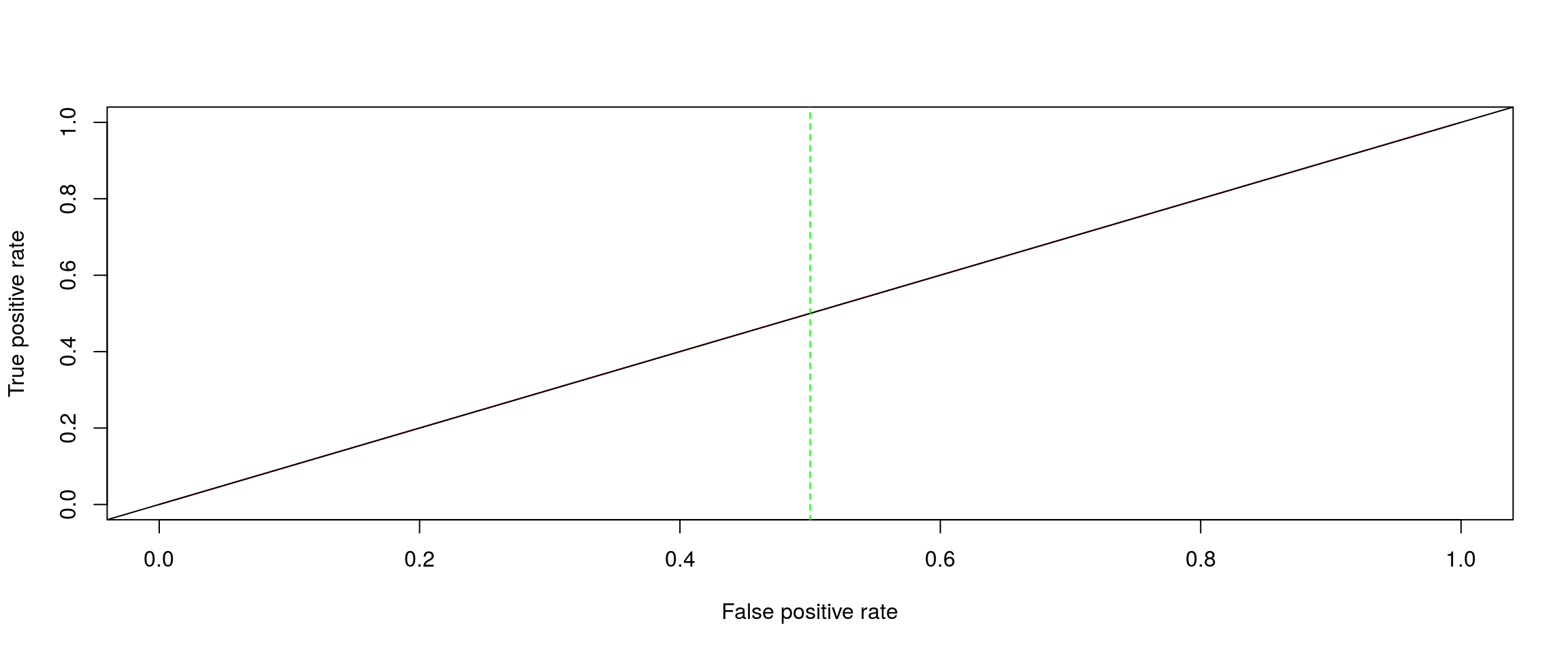

Naiwny Klasyfikator Bayesa

model_bayes <- naiveBayes(bcr_patient_barcode~.,
                          data=BRCA.rnaseq.tumor.first[1:1000,-do_wywalenia], laplace=0.2)

bayes_prawd <- predict(model_bayes, newdata=BRCA.rnaseq.tumor.first[1001:1212,-do_wywalenia], 
                       type="raw")[,2]
klasy_bayes_pred <- ifelse( bayes_prawd >0.5, 1, 0)
tabela(klasy_bayes_pred, as.integer(BRCA.rnaseq.tumor.first[1001:1212,1])) -> tab_bayes
tab_bayes

               klasy_prawdziwe
predykcja_klasy   0   1
              0 200   0
              1   1  11

precyzja(tab_bayes)

[1] 1

czulosc(tab_bayes)

[1] 0.9166667

procent(tab_bayes)

[1] 99.5283

roc(bayes_prawd, as.integer(BRCA.rnaseq.tumor.first[1001:1212,1]))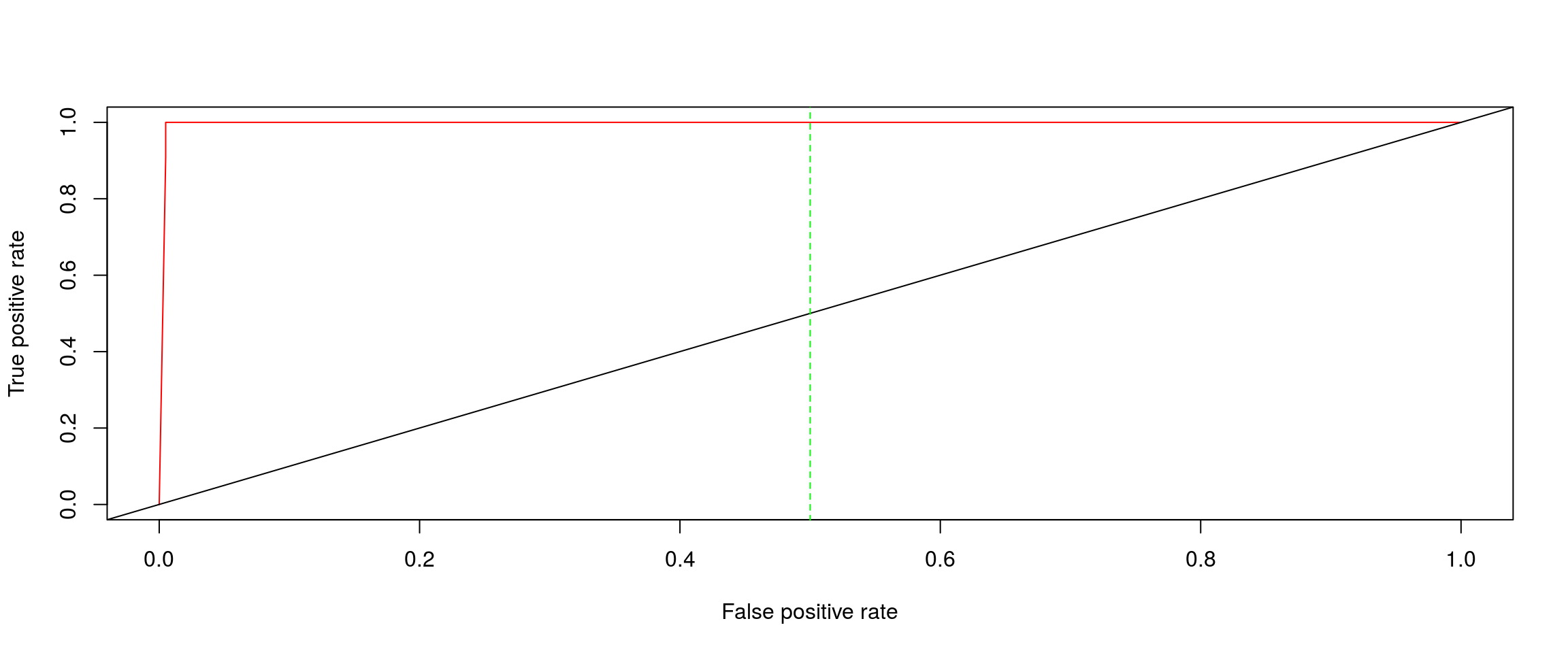

Gdzie szukać więcej algorytmów/kodów

• https://github.com/MarcinKosinski/DataMiningProject/tree/master/scripts_Rnw
• http://grupawp.github.io/codepot-workshop-2015/06_klasyfikacja.html
• caret : http://topepo.github.io/caret/training.html
• xgboost : https://github.com/mi2-warsaw/SER/blob/master/SER_XIX/xgboost.R

Session info:

sessionInfo()

R version 3.3.0 (2016-05-03)
Platform: x86_64-pc-linux-gnu (64-bit)
Running under: Ubuntu 14.04.4 LTS

locale:
 [1] LC_CTYPE=pl_PL.UTF-8          LC_NUMERIC=C                  LC_TIME=pl_PL.UTF-8           LC_COLLATE=pl_PL.UTF-8       
 [5] LC_MONETARY=pl_PL.UTF-8       LC_MESSAGES=pl_PL.UTF-8       LC_PAPER=pl_PL.UTF-8          LC_NAME=pl_PL.UTF-8          
 [9] LC_ADDRESS=pl_PL.UTF-8        LC_TELEPHONE=pl_PL.UTF-8      LC_MEASUREMENT=pl_PL.UTF-8    LC_IDENTIFICATION=pl_PL.UTF-8

attached base packages:
[1] stats     graphics  grDevices utils     datasets  methods   base     

other attached packages:
 [1] knitr_1.13                   e1071_1.6-7                  ROCR_1.0-7                   gplots_3.0.1                 glmnet_2.0-5                
 [6] foreach_1.4.3                Matrix_1.2-6                 Boruta_5.0.0                 ranger_0.4.0                 FSelector_0.20              
[11] survival_2.39-4              survminer_0.2.1.900          ggplot2_2.1.0                tidyr_0.4.1                  RTCGA.clinical_20151101.2.0 
[16] RTCGA.mutations_20151101.2.0 RTCGA.rnaseq_20151101.2.0    RTCGA_1.2.2                  dplyr_0.4.3                  rmarkdown_0.9.6             

loaded via a namespace (and not attached):
 [1] Rcpp_0.12.5         lattice_0.20-33     RWeka_0.4-27        class_7.3-14        gtools_3.5.0        assertthat_0.1      digest_0.6.9       
 [8] R6_2.1.2            plyr_1.8.4          chron_2.3-47        evaluate_0.9        httr_1.1.0          RWekajars_3.9.0-1   lazyeval_0.1.10    
[15] data.table_1.9.6    gdata_2.17.0        labeling_0.3        devtools_1.11.1     splines_3.3.0       stringr_1.0.0       pander_0.6.0       
[22] munsell_0.4.3       htmltools_0.3.5     gridExtra_2.2.1     codetools_0.2-14    randomForest_4.6-12 XML_3.98-1.4        withr_1.0.1        
[29] bitops_1.0-6        grid_3.3.0          gtable_0.2.0        DBI_0.4-1           magrittr_1.5        formatR_1.4         scales_0.4.0       
[36] KernSmooth_2.23-15  stringi_1.1.1       viridis_0.3.4       ggthemes_3.0.3      xml2_0.1.2          iterators_1.0.8     tools_3.3.0        
[43] entropy_1.2.1       purrr_0.2.1         parallel_3.3.0      yaml_2.1.13         colorspace_1.2-6    caTools_1.17.1      rvest_0.3.1        
[50] memoise_1.0.0       rJava_0.9-8